Want to make your Excel sheet smarter? Here’s an amazing trick to automatically highlight rows based on a city name! This method is simple, quick, and perfect for managing large data sets.
✅ Why Use This Trick?
- Quickly find data for any city.
- No need to scroll through long sheets.
- Save time and improve productivity.
📋 Step-by-Step Guide to Highlight Rows:
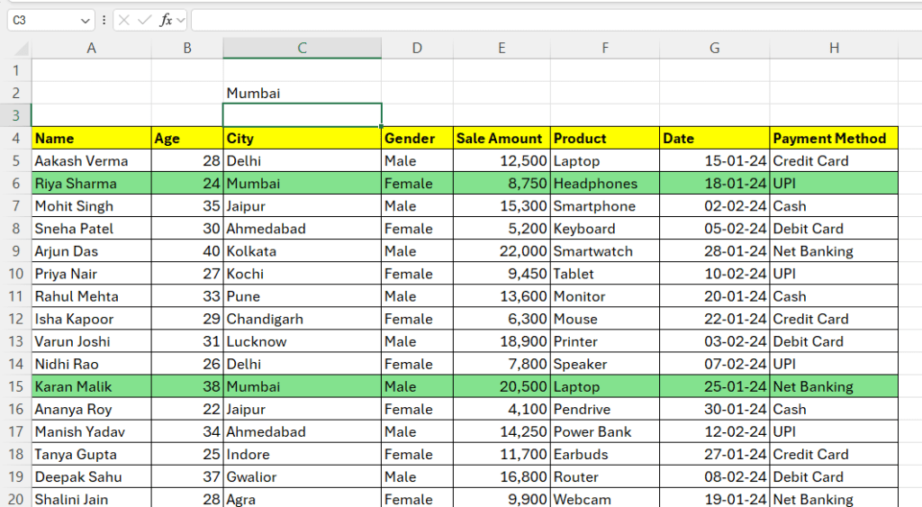
- Select Your Data:
Highlight the range where your data is present (e.g., A4:H33). - Go to Conditional Formatting:
- Click on the “Home” tab.
- Select “Conditional Formatting” → “New Rule”.
- Choose the Formula Option:
- Click on “Use a formula to determine which cells to format”.
- Enter the Formula:
=$C4=$C$2- $C4 refers to the City column (adjust if your city is in a different column).
- $C$2 is the cell where you’ll type the city name (like “Delhi”).
- Set the Format:
- Click on “Format”.
- Choose a color to highlight the matching rows.
- Click OK.
- Type the City Name:
- In C2, type the city name (e.g., “Delhi”).
- Instantly, all rows with “Delhi” will be highlighted automatically!
🎯 Bonus Tip:
You can change the city name anytime in C2, and Excel will update the highlights instantly. Super cool, right? 😎
🚀 Download the Practice Sheet:
Want to try it yourself?
🔍 SEO Keywords:
- How to highlight rows in Excel based on cell value
- Excel conditional formatting by city name
- Highlight multiple rows in Excel automatically
- Excel tricks for data analysis
- Easy Excel tips for beginners
Stay tuned with SeekheIndia for more Excel hacks! 😊